这一篇是阶段性的总结。
下载数据
这次还是用mothur的测试数据。我把样本信息也弄好了。
wget https://raw.githubusercontent.com/pzweuj/practice/master/R/DADA2_workflow2/Rawdata/Rawdata.tar
tar -xvf Rawdata.tar
dada2
接下来走一套dada2的流程。
library(dada2) # loads DADA2

list.files("Filtdata")

# setting a few variables we're going to use
fnFs <- sort(list.files("Filtdata", pattern="_sub_R1_trim.fq.gz", full.names=TRUE))
fnRs <- sort(list.files("Filtdata", pattern="_sub_R2_trim.fq.gz", full.names=TRUE))

sample.names <- sapply(strsplit(basename(fnFs), "_"), `[`, 1)

filtFs <- file.path("Cleandata", paste0(sample.names, "_sub_R1_filtered.fq.gz"))
filtRs <- file.path("Cleandata", paste0(sample.names, "_sub_R2_filtered.fq.gz"))
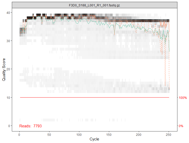
画几张质量图
plotQualityProfile(fnFs[1])
plotQualityProfile(fnRs)
plotQualityProfile(fnFs[17:20])
过滤
out <- filterAndTrim(
fnFs, filtFs, fnRs, filtRs, truncLen=c(240, 160),
maxN=0, maxEE=c(2, 2), truncQ=2, rm.phix=TRUE,
compress=TRUE, multithread=TRUE # 在windows下,multithread设置成FALSE
)
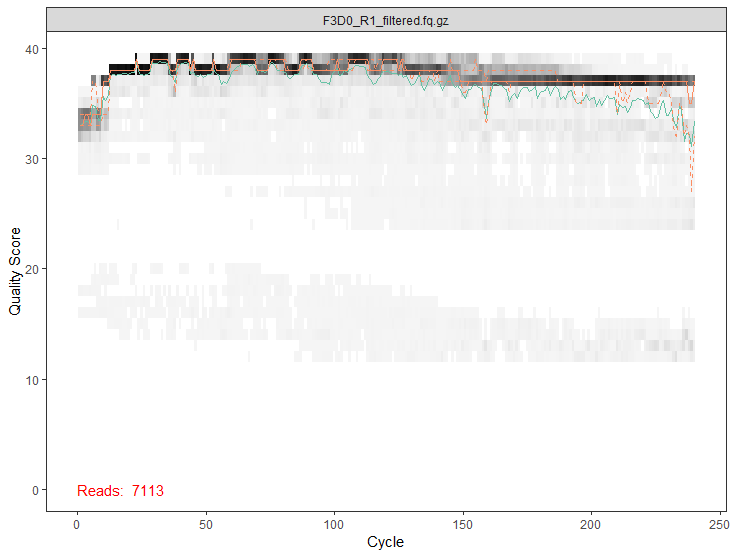
# 画一下过滤后的
plotQualityProfile(filtFs[1])
计算错误率模型
# 分别计算正向和反向
errF <- learnErrors(filtFs, multithread=TRUE)
errR <- learnErrors(filtRs, multithread=TRUE)
# 画出错误率统计图
plotErrors(errF, nominalQ=TRUE)
plotErrors(errR, nominalQ=TRUE)
消除误差
# 下面其实是一个批量的操作,如果是处理大文件,内存可能不足,更好的做法是一个一个样本的进行
derepFs <- derepFastq(filtFs, verbose=TRUE)
derepRs <- derepFastq(filtRs, verbose=TRUE)
# 用sample.names来改名
names(derepFs) <- sample.names
names(derepRs) <- sample.names
dada2核心算法
# 从头OTU方法必须在处理之前对样本进行聚类,因为样本之间没有聚类标签不一致且无法比较,即样本1中的OTU1和样本2中的OTU1可能不相同。
# 而DADA2可以更精确地解析序列变异,可以独立处理然后组合。
dadaFs <- dada(derepFs, err=errF, multithread=TRUE)
dadaRs <- dada(derepRs, err=errR, multithread=TRUE)
合并双端
mergers <- mergePairs(dadaFs, derepFs, dadaRs, derepRs, verbose=TRUE)
# 构造列表
seqtab <- makeSequenceTable(mergers)
dim(seqtab)
# 检测长度分布
table(nchar(getSequences(seqtab)))
去除嵌合体
seqtab.nochim <- removeBimeraDenovo(seqtab, method="consensus", multithread=T, verbose=T)
dim(seqtab.nochim)
sum(seqtab.nochim)/sum(seqtab)
物种分类
# 这里是使用silva数据库进行注释。
# 然后把特征序列都提出来,在对这些序列进行命名,命名的方式为“ASV_x”。
taxa <- assignTaxonomy(seqtab.nochim, "Database/silva_nr_v132_train_set.fa.gz", multithread=T, tryRC=T)
输出DADA2结果
asv_seqs <- colnames(seqtab.nochim)
asv_headers <- vector(dim(seqtab.nochim)[2], mode="character")

for (i in 1:dim(seqtab.nochim)[2]) {
  asv_headers[i] <- paste(">ASV", i, sep="_")
}

# 这一步输出三个文件,一个是把特征序列都放在一起的fasta文件,一个是注释文件,一个是counts数文件。
# fasta:
asv_fasta <- c(rbind(asv_headers, asv_seqs))
write(asv_fasta, "ASV/ASVs.fa")

# count table:
asv_count <- t(seqtab.nochim)
row.names(asv_count) <- sub(">", "", asv_headers)
write.table(asv_count, "ASV/ASVs_counts.txt", sep="\t", quote=F)

# tax table:
asv_taxa <- taxa
row.names(asv_taxa) <- sub(">", "", asv_headers)
write.table(asv_taxa, "ASV/ASVs_taxonomy.txt", sep="\t", quote=F)
以上过程,完成了整个dada2流程,生成了3个文件。
读入文件以及需要的包
library("phyloseq")
library("vegan")
library("DESeq2")
library("ggplot2")
library("dendextend")
#library("tidyr")
#library("viridis")
#library("reshape")

countdata <- read.table("ASV/ASVs_counts.txt", header=T, row.names=1, check.names=F)
taxdata <- as.matrix(read.table("ASV/ASVs_taxonomy.txt", header=T, row.names=1, check.names=F, na.strings="", sep="\t"))

sample_info <- read.table("Rawdata/sample_info.txt", header=T, row.names=1, check.names=F)
初步处理
# 排序
# ord_col <- as.numeric(sapply(names(countdata), FUN=function(x){strsplit(x, "F3D")[[1]][2]}))
# countdata <- countdata[order(ord_col)]

# ord_row <- as.numeric(sapply(row.names(sample_info), FUN=function(x){strsplit(x, "F3D")[[1]][2]}))
# sample_info <- sample_info[order(ord_row),]

# 设置颜色
sample_info$color[sample_info$time == "Early"] <- "green"
sample_info$color[sample_info$time == "Late"] <- "red"

# 创建新的phyloseq对象
count_phy <- otu_table(countdata, taxa_are_rows=T)
tax_phy <- tax_table(taxdata)
sample_info_phy <- sample_data(sample_info)
ASV_physeq <- phyloseq(count_phy, tax_phy, sample_info_phy)
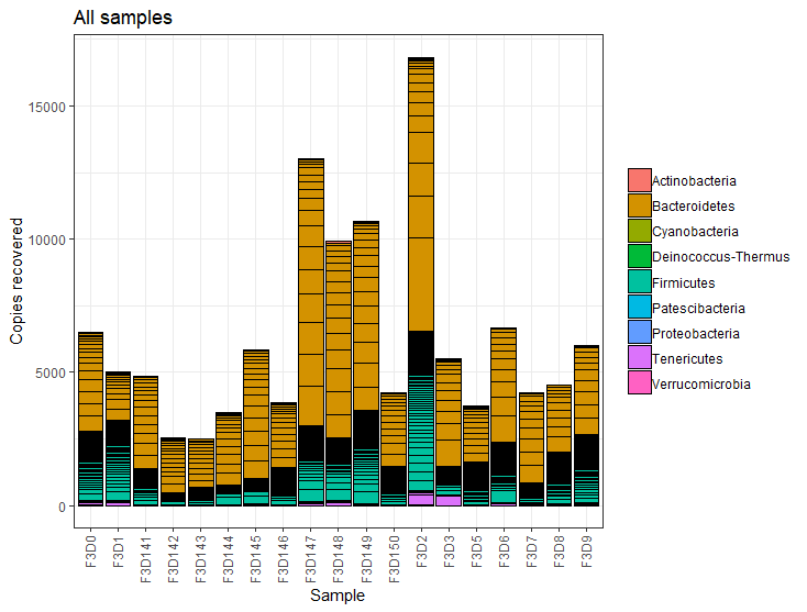
物种丰富度柱状图
plot_bar(ASV_physeq, fill="Phylum") +
  theme_bw() +
  theme(axis.text.x=element_text(angle=90, vjust=0.4, hjust=1), legend.title=element_blank()) +
  labs(x="Sample", y="Copies recovered", title="All samples")
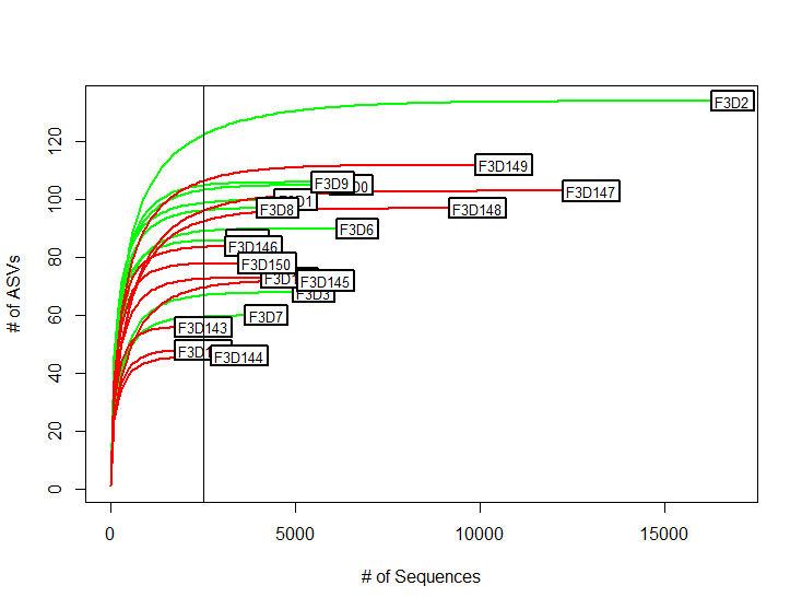
Alpha分析
# 稀释曲线
rarecurve(t(countdata), step=100, col=sample_info$color, lwd=2, ylab="# of ASVs", xlab="# of Sequences")
abline(v=(min(rowSums(t(countdata)))))
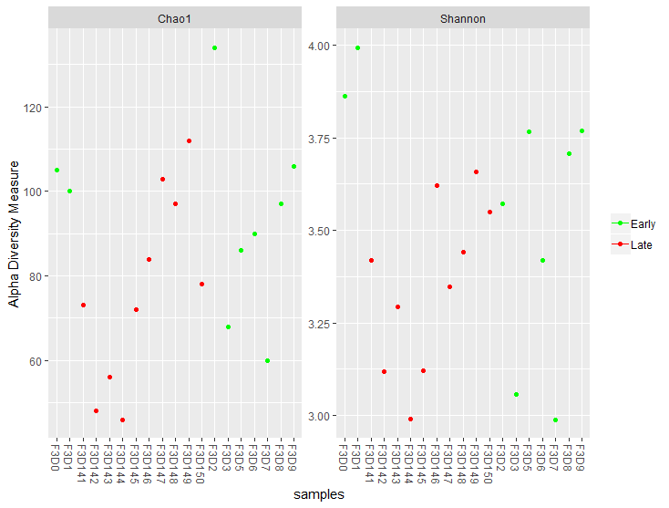
# 画出Chao1和Shannon
# 横坐标为样本
plot_richness(ASV_physeq, color="time", measures=c("Chao1", "Shannon")) +
  scale_color_manual(values=unique(sample_info$color[order(sample_info$time)])) +
  theme(legend.title = element_blank())
# 横坐标为状态
plot_richness(ASV_physeq, x="dpw", color="time", measures=c("Chao1", "Shannon")) +
  scale_color_manual(values=unique(sample_info$color[order(sample_info$time)])) +
  theme(legend.title = element_blank())
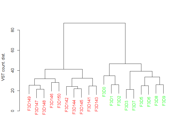
Beta分析
# 使用DESeq2进行差异分析
deseq_counts <- DESeqDataSetFromMatrix(countdata, colData = sample_info, design = ~time)
deseq_counts_vst <- varianceStabilizingTransformation(deseq_counts)

# 生成表格
vst_trans_count <- assay(deseq_counts_vst)

# 计算出差异矩阵
dist_count <- dist(t(vst_trans_count))

# 聚类
clust_count <- hclust(dist_count, method="ward.D2")
dend_count <- as.dendrogram(clust_count, hang=0.1)
dend_cols <- sample_info$color[order.dendrogram(dend_count)]
labels_colors(dend_count) <- dend_cols

# 画出树
plot(dend_count, ylab="VST count. dist.")
# 使用差异矩阵
vst_count_phy <- otu_table(vst_trans_count, taxa_are_rows=T)
vst_physeq <- phyloseq(vst_count_phy, sample_info_phy)

# 使用phyloseq画PCoA图
vst_pcoa <- ordinate(vst_physeq, method="MDS", distance="euclidean")
eigen_vals <- vst_pcoa$values$Eigenvalues

# PCoA图
plot_ordination(vst_physeq, vst_pcoa, color="time") +
  labs(col="dpw") + geom_point(size=1) +
  geom_text(aes(label=rownames(sample_info), hjust=0.3, vjust=-0.4)) +
  coord_fixed(sqrt(eigen_vals[2]/eigen_vals[1])) + ggtitle("PCoA") +
  scale_color_manual(values=unique(sample_info$color[order(sample_info$time)])) +
  theme(legend.position="none")
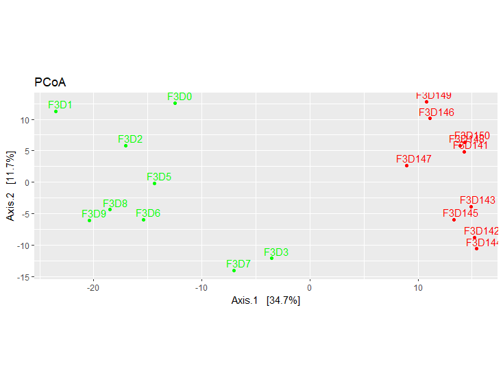
可以看出随着前9天和后9天的组间差异还是很明显的。
至此,扩增子的学习暂告一段落了。