背景
加权基因共表达网络分析(Weighted Gene Co-Expression Network Analysis, WGCNA)。该分析方法旨在寻找协同表达的基因模块(module),在该方法中module被定义为一组具有类似表达趋势的基因集,如果这些基因在一个生理过程或不同组织中总是具有相类似的表达变化,就有理由认为它们在功能上是相关的,可以把它们定义为一个module。
分析标准:样本最好在15个以上,样本分组差异不应太大。
数据预处理
采用RNA-seq数据,先过滤掉所有样本中均低表达的基因,再过滤掉所有样本中几乎没有差异的基因(最好不要只留差异基因)。按照一般做法,分析基因的表达丰度用TPM,分析差异基因用counts,WGCNA比较偏向于分析表达丰度,所以采用TPM。
接下来采用:Tutorials for the WGCNA package这个官方教程。
点击这里下载数据。
这些数据是来自雌性小鼠的肝脏表达数据。
# install.packages("WGCNA")
# 设置将strings不要转成factors
options(stringsAsFactors=F)

# 读入表达数据
femData <- read.csv("LiverFemale3600.csv")
# 查看数据
dim(femData)
names(femData)

# 数据初步处理
# 提取出表达数据
datExpr0 <- as.data.frame(t(femData[, -c(1:8)]))
names(datExpr0) <- femData$substanceBXH
rownames(datExpr0) <- names(femData)[-c(1:8)]

# 样本聚类检查离群值(就是树上特别不接近的)
gsg <- goodSamplesGenes(datExpr0, verbose=3)
# 是true的话说明所有genes都通过了筛选
gsg$allOK

if (!gsg$allOK){
  if (sum(!gsg$goodGenes)>0)
    printFlush(paste("Removing genes:", paste(names(datExpr0)[!gsg$goodGenes], collapse=", ")))
  if (sum(!gsg$goodSamples)>0)
    printFlush(paste("Removing samples:", paste(rownames(datExpr0)[!gsg$goodSamples], collapse=", ")))
  datExpr0 <- datExpr0[gsg$goodSamples, gsg$goodGenes]
}

# 画图来看是否有特别离群的
sampleTree <- hclust(dist(datExpr0), method="average")
sizeGrWindow(12, 9)
par(cex=0.6)
par(mar=c(0,4,2,0))
plot(sampleTree, main="Sample clustering to detect outliers", sub="", xlab="", cex.lab=1.5,
     cex.axis=1.5, cex.main=2)
abline(h=15, col="red")
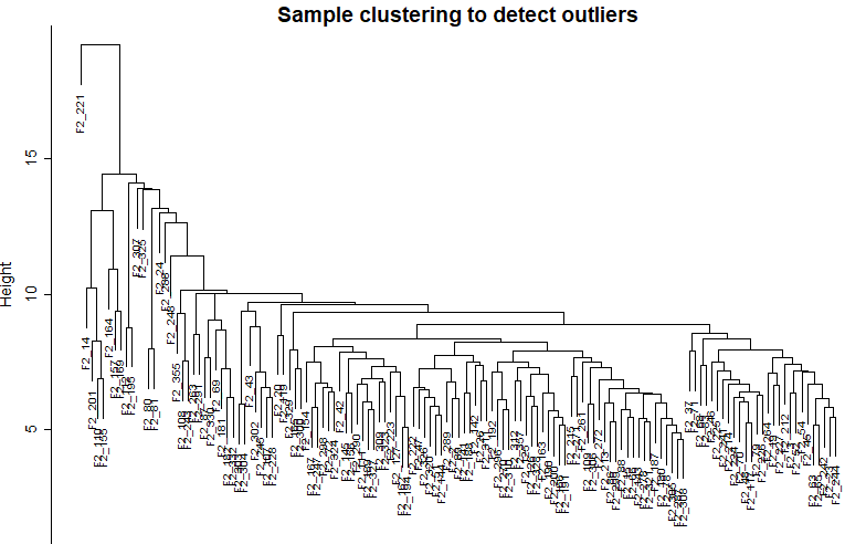
明显有一个离群的样本。
# 把离群的修剪掉
clust <- cutreeStatic(sampleTree, cutHeight=15, minSize=10)
table(clust)
keepSamples <- (clust==1)
datExpr <- datExpr0[keepSamples, ]
nGenes <- ncol(datExpr)
nSamples <- nrow(datExpr)

# 只保留需要的信息
allTraits <- traitData[, -c(31, 16)]
allTraits <- allTraits[, c(2, 11:36)]
dim(allTraits)
names(allTraits)

# 使两个数据框的行名一致
femaleSamples <- rownames(datExpr)
traitRows <- match(femaleSamples, allTraits$Mice)
datTraits <- allTraits[traitRows, -1]
rownames(datTraits) <- allTraits[traitRows, 1]

# 清理,释放内存
collectGarbage()

# 作性状与样本的关系热图
sampleTree2 <- hclust(dist(datExpr), method="average")
traitColors <- numbers2colors(datTraits, signed=F)
plotDendroAndColors(sampleTree2, traitColors,
                    groupLabels=names(datTraits),
                    main="Sample dendrogram and trait heatmap")

# 保存预处理完成的数据
save(datExpr, datTraits, file="dataInput.RData")
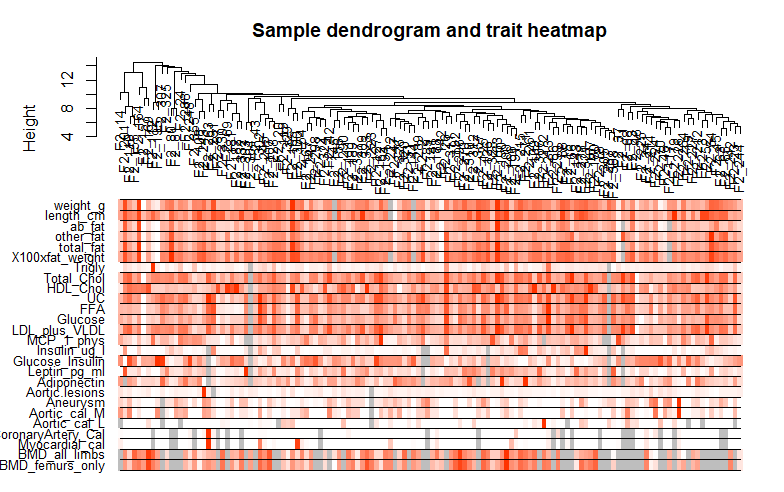
这个图可以看出不同的样本间,性状的一致性。
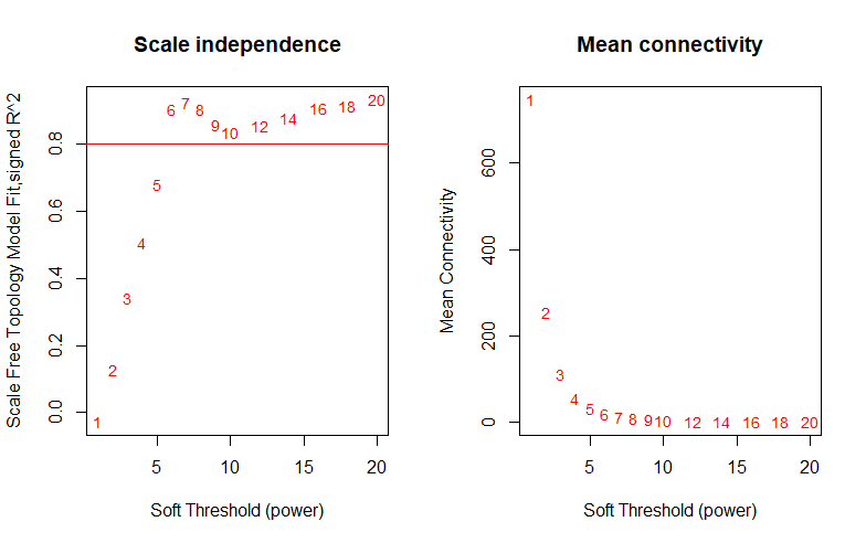
求软阈值
一开始数据是一个基因表达矩阵,然后接着需要构建相关性矩阵。相关性矩阵有两种,分别是Signed相关性矩阵(区分正相关和负相关)和Unsigned相关性矩阵(不区分正负)。接着需要将相关性矩阵构建成邻接矩阵。由于设置阈值时具有人为干扰,WGCNA推荐使用软阈值。原则上,需要尽可能接近无尺度网络(Scale independence第一次达到0.8以上),尽可能保留连通性信息。
# 允许使用最大线程
allowWGCNAThreads()
# 或者直接指定线程数
enableWGCNAThreads(nThreads=16)

# 软阈值的预设范围
powers <- c(c(1:10), seq(from=12, to=20, by=2))
# 自动计算推荐的软阈值
sft <- pickSoftThreshold(datExpr, powerVector=powers, verbose=5, networkType="unsigned")
# 推荐值。如果是NA,就需要画图来自己挑选
sft$powerEstimate

# 作图
sizeGrWindow(9, 5)
par(mfrow=c(1, 2))
cex1 <- 0.9
plot(sft$fitIndices[, 1], -sign(sft$fitIndices[, 3])*sft$fitIndices[, 2],
     xlab="Soft Threshold (power)", ylab="Scale Free Topology Model Fit,signed R^2", type="n",
     main=paste("Scale independence"))
text(sft$fitIndices[, 1], -sign(sft$fitIndices[, 3])*sft$fitIndices[, 2],
     labels=powers, cex=cex1, col="red")
abline(h=0.80, col="red")
plot(sft$fitIndices[, 1], sft$fitIndices[, 5],
     xlab="Soft Threshold (power)", ylab="Mean Connectivity", type="n",
     main=paste("Mean connectivity"))
text(sft$fitIndices[, 1], sft$fitIndices[, 5], labels=powers, cex=cex1, col="red")

# 如果是NA,此时就需要根据图来自己指定数值了
sft$powerEstimate <- 6
构建矩阵
最后构建拓扑重叠矩阵(TOM矩阵),目的是引入中间节点。因为构建邻接矩阵采用pearson相关,只描述线性关系,可能会漏掉一些非线性相关的基因。
# 构建网络
# deepSplit是生成模块的梯度,从[0:4]中选择,越大模块越多
# minModuleSize最小模块的基因数目
# mergeCutHeight是合并相似的模块的合并系数,是通过主成分分析出来的
# mumericLabels 已数字命名模块
# nThreads 线程数,当设置为0时使用最大线程
net <- blockwiseModules(datExpr, corType="pearson",
                        power=sft$powerEstimate,
                        TOMType="unsigned", saveTOMs=TRUE, saveTOMFileBase="femaleMouseTOM",
                        deepSplit=2, minModuleSize=30,
                        reassignThreshold=0, mergeCutHeight=0.25,
                        numericLabels=T, pamRespectsDendro=F, nThreads=0,
                        verbose=3)

# 查看每个模块的基因数,其中0模块下为没有计算进入模块的基因数
table(net$colors)
结果可视化
sizeGrWindow(12, 9)
# 把模块编号转成颜色
mergedColors <- labels2colors(net$colors)
plotDendroAndColors(net$dendrograms[[1]], mergedColors[net$blockGenes[[1]]],
                    "Module colors",
                    dendroLabels=F, hang=0.03,
                    addGuide=T, guideHang=0.05)
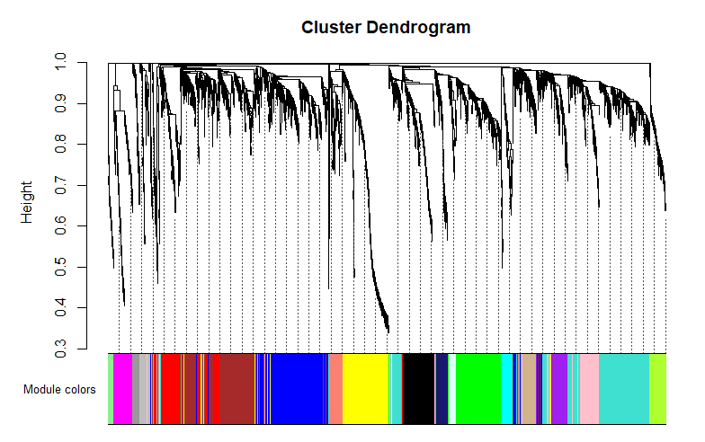
上图中,树图每个分支是一个基因,下面每一种颜色代表一个模块。
保存结果
# 计算模块特征向量MEs
moduleLabels <- net$colors
moduleColors <- labels2colors(net$colors)
MEs <- net$MEs
geneTree <- net$dendrograms[[1]]
# 保存数据
save(MEs, moduleLabels, moduleColors, geneTree,
     file="networkConstruction-auto.RData")
模块与性状关联
做主成分分析,用PC1代表模块的指标(用模块特征向量ME表示)。计算ME与性状的相关系数,再将相关系数用热图表示出来。
nGenes <- ncol(datExpr)
nSamples <- nrow(datExpr)

# 重新计算MEs
MEs0 <- moduleEigengenes(datExpr, moduleColors)$eigengenes
MEs <- orderMEs(MEs0)
# 主成分向量和性状的关联,pearson校正
moduleTraitCor <- cor(MEs, datTraits, use="p")
moduleTraitPvalue <- corPvalueStudent(moduleTraitCor, nSamples)

# 画出模块和性状的关联热图
sizeGrWindow(10, 6)
# 把校正值和p值写在一起
textMatrix <-  paste(signif(moduleTraitCor, 2), "\n(",
                     signif(moduleTraitPvalue, 1), ")", sep="")
dim(textMatrix) <- dim(moduleTraitCor)
par(mar=c(6, 8.5, 3, 3))
# 画图
labeledHeatmap(Matrix=moduleTraitCor,
               xLabels=names(datTraits),
               yLabels=names(MEs),
               ySymbols=names(MEs),
               colorLabels=F,
               colors=greenWhiteRed(50),
               textMatrix=textMatrix,
               setStdMargins=F,
               cex.text=0.5,
               zlim=c(-1,1),
               main=paste("Module-trait relationships"))
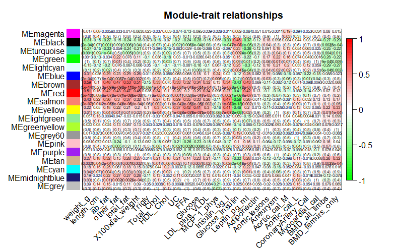
上图已经能看出每个性状与各个模块的关联性。
计算模组与性状/基因与性状的相关性
得到相关性最高的模块后,计算模块内单独的基因与模块的相关性(MM),也可以计算单独的基因与性状的相关性(GS)。
## 计算模组
modNames <- substring(names(MEs), 3)
# 计算MM
geneModuleMembership <- as.data.frame(cor(datExpr, MEs, use="p"))
MMPvalue <- as.data.frame(corPvalueStudent(as.matrix(geneModuleMembership), nSamples))
names(geneModuleMembership) <- paste("MM", modNames, sep="")
names(MMPvalue) <- paste("p.MM", modNames, sep="")
# 计算GS
geneTraitSignificance <- as.data.frame(cor(datExpr, datTraits, use="p"))
GSPvalue <- as.data.frame(corPvalueStudent(as.matrix(geneTraitSignificance), nSamples))
names(geneTraitSignificance) <- paste("GS.", names(datTraits), sep="")
names(GSPvalue) <- paste("p.GS.", names(datTraits), sep="")

# 输出
geneInfo <- cbind(geneModuleMembership, MMPvalue, geneTraitSignificance, GSPvalue)
write.table(geneInfo, file="geneInfo.txt", sep="\t", quote=F)
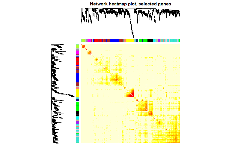
可视化
画模块之间的热图。
# power是之前的软阈值
TOM <- TOMsimilarityFromExpr(datExpr, power=sft$powerEstimate)
dissTOM <- 1 - TOM
#为了更显著,用7次方
plotTOM <- dissTOM^7
diag(plotTOM) <- NA
TOMplot(plotTOM, geneTree, moduleColors, main="Network heatmap plot, all genes")


# 随机抽,自行取值
nSelect <- 400
set.seed(10)
select <- sample(nGenes, size=nSelect)
selectTOM <- dissTOM[select, select]

# 重新聚类
selectTree <- hclust(as.dist(selectTOM), method="average")
selectColors <- moduleColors[select]
# 绘图
plotDiss <- selectTOM^7
diag(plotDiss) <- NA
TOMplot(plotDiss, selectTree, selectColors, main="Network heatmap plot, selected genes")
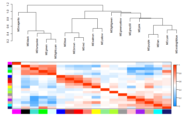
# 模块聚类与热图
plotEigengeneNetworks(MEs, "", marDendro=c(0, 4, 1, 2),
                      marHeatmap=c(3, 4, 1, 2), cex.lab=0.8,
                      plotDendrograms=T, plotHeatmaps=T,
                      xLabelsAngle=90)
还可以使用Cytoscape进行可视化。
# 选择可视化模块
modules <- c("brown")
# 得到基因ID
probes <- colnames(datExpr)
inModule <- is.finite(match(moduleColors, modules))
modProbes <- probes[inModule]
# 得到候选基因的TOM
modTOM <- TOM[inModule, inModule]
# 命名
dimnames(modTOM) <- list(modProbes, modProbes)
# 输出cytoscape
cyt <- exportNetworkToCytoscape(modTOM,
                                edgeFile=paste("brown-cyto-edge-", paste(modules, collapse="-"), ".txt", sep=""),
                                nodeFile=paste("brown-cyto-nodes-", paste(modules, collapse="-"), ".txt", sep=""),
                                weighted=T, threshold = 0.02,
                                nodeNames=modProbes,
                                nodeAttr=moduleColors[inModule])
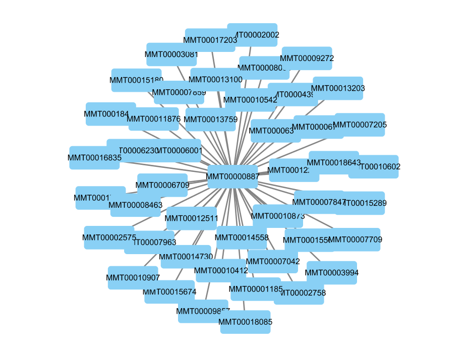
上图只是举例,由于edges文件很大,几乎每两个基因都存在关系。因此在此前最好还是做多一部筛选。或者选取一个基因或少许基因作为seed。