跟着大佬学习一下机器学习100-Days-Of-ML。
Day 4 逻辑回归
第4天简单的一张图说明逻辑回归

Day5 逻辑回归
逻辑回归(Logistic Regression)是一种用于解决二分类(0 or 1)问题的机器学习方法,用于估计某种事物的可能性。比如某用户购买某商品的可能性,某病人患有某种疾病的可能性,以及某广告被用户点击的可能性等。 注意,这里用的是“可能性”,而非数学上的“概率”,logisitc回归的结果并非数学定义中的概率值,不可以直接当做概率值来用。该结果往往用于和其他特征值加权求和,而非直接相乘。(credit to 知乎)
Day6 逻辑回归
这一天的内容是使用逻辑回归的方法,从数据中预测会购买豪华SUV的潜在客户。 使用的数据在这里。
预处理
修改了一点,避免出现Warning。
import pandas as pd
import numpy as np
import matplotlib.pyplot as plt

# 导入
dataset = pd.read_csv("Social_Network_Ads.csv")
# 年龄-收入
X = dataset.iloc[:, [2, 3]].values
# 购买情况
Y = dataset.iloc[:, 4].values

# 将数据集分成训练集和测试集
from sklearn.model_selection import train_test_split
X_train, X_test, y_train, y_test = train_test_split(X, Y, test_size=0.25, random_state=0)

# 特征缩放
from sklearn.preprocessing import StandardScaler
sc = StandardScaler()

X_train = X_train.astype(np.float64)
X_test = X_test.astype(np.float64)

X_train = sc.fit_transform(X_train)
X_test = sc.transform(X_test)
逻辑回归模型
from sklearn.linear_model import LogisticRegression
classifier = LogisticRegression(solver="liblinear")
classifier.fit(X_train, y_train)
预测
y_pred = classifier.predict(X_test)
评估预测
# 生成混淆矩阵
from sklearn.metrics import confusion_matrix
cm = confusion_matrix(y_test, y_pred)
# 可视化
from matplotlib.colors import ListedColormap
X_set, y_set = X_train, y_train
X1, X2 = np.meshgrid(np.arange(start=X_set[:,0].min()-1, stop=X_set[:, 0].max()+1, step=0.01),
np.arange(start=X_set[:, 1].min()-1, stop=X_set[:, 1].max()+1, step=0.01))
plt.contourf(X1, X2, classifier.predict(np.array([X1.ravel(), X2.ravel()]).T).reshape(X1.shape),
alpha = 0.75, cmap = ListedColormap(("red", "green")))
plt.xlim(X1.min(), X1.max())
plt.ylim(X2.min(), X2.max())
for i, j in enumerate(np.unique(y_set)):
plt.scatter(X_set[y_set==j,0], X_set[y_set==j,1],
c = ListedColormap(("red", "green"))(i), label=j)
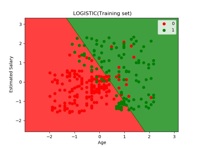
plt.title(" LOGISTIC(Training set)")
plt.xlabel(" Age")
plt.ylabel(" Estimated Salary")
plt.legend()
plt.show()
X_set, y_set = X_test, y_test
X1, X2=np.meshgrid(np.arange(start=X_set[:, 0].min()-1, stop=X_set[:, 0].max()+1, step=0.01),
np.arange(start=X_set[:, 1].min()-1, stop=X_set[:, 1].max()+1, step=0.01))
plt.contourf(X1, X2, classifier.predict(np.array([X1.ravel(), X2.ravel()]).T).reshape(X1.shape),
alpha=0.75, cmap=ListedColormap(("red", "green")))
plt.xlim(X1.min(), X1.max())
plt.ylim(X2.min(), X2.max())
for i, j in enumerate(np.unique(y_set)):
plt.scatter(X_set[y_set==j, 0], X_set[y_set==j, 1],
c=ListedColormap(("red", "green"))(i), label=j)
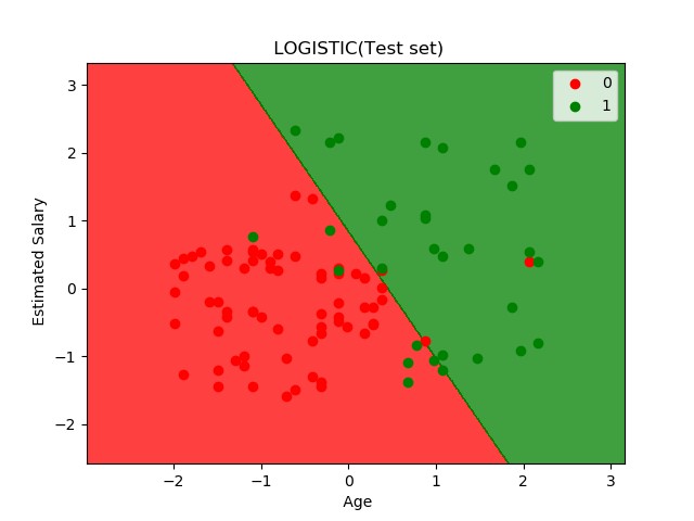
plt.title(" LOGISTIC(Test set)")
plt.xlabel(" Age")
plt.ylabel(" Estimated Salary")
plt.legend()
plt.show()
最终出图